I’ve been experimenting with measuring pitch change due to bore perturbation and would like to compare notes (ba-dum!). I want to get an idea of how accurate Benade’s W-Curve method is. I’m also comparing the results with a method of Nederveen (as described by Prairie).
Some disclaimers up front:
–This isn’t a sophisticated physics-lab type of thing; more like a science fair project out in the garage.
–The algorithms don’t involve tone holes, just the bore profile (unlike more sophisticated approaches used by Dickens, WIDesigner, etc.)
The goal here is not to have a setup to test complex scenarios on real instruments. Rather, it is to build relatively simple test cases to vet the algorithms and–especially–their software implementations. After that, the complex scenarios can best be done in software.
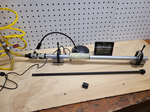
Here’s a photo of the setup. I’m basically blowing a low whistle with compressed air, and inserting sleeves to constrict the bore. Later I plan to test some conical bores as well.
I’ve just started measuring, so I haven’t drawn any conclusions yet. Here’s an initial result–the algorithms seem to be good within a cent or two…
More detail is available at https://www.forbesflutes.com/research/ under the items “A Simple Setup for Measuring Pitch Change” and “Bore Perturbation: Comparing Algorithms with Measurements”.
So, has anyone tried something similar? How did it work out? I’d appreciate any references to studies comparing theory with actual pitch measurements; they seem a bit hard to find…
Yes, that is indeed the Perturbation Positioner (aka a plastic rod with washers on the ends). I get tired of typing “perturbation” so I abbreviate it “ptb”
5. Is the small black item in the foreground a ptb ?
Yup, that’s the short section of plastic tube that is the bore perturbation.
6 what is the zero-reference for the graph’s x-scale ? (e.g. window or foot)
Sorry for not being clearer on that. The 0 is the window (blowing edge). The distance is to the center of the sleeve. When positioning the sleeve I actually measure from the foot because it is more precise, then convert that into a distance from the window for the graph. The graph only shows the bottom half of the instrument. If it was starting from zero, you would see the curves are the bell-shaped “W curves” that Benade illustrates in Fundamentals of Musical Acoustics.
I wish my “garage” were that neat + tidy !
Yeah, me too I must confess that for the picture I grabbed a couple of pieces of pegboard to hide the actual mess behind the setup…
[This is an edited version of the post that removes some errors that were due to a software bug…]
Trill,
The ID of the tube is .762" and the ptb bushing is ID .705" x .884" long. It’s the area that’s important acoustically, so the area ratio is (.705/.762)^2 = .86 so that’s a 14% change–fairly large. I wanted to get a large change that would show up against random variation. As it turns out, the measurements look fairly clean, so I could have used less ptb. As you requested, I made some more measurements closer to the fipple:
The outer vertical dashed lines show the acoustic extent of the bore–i.e. with end corrections added–and the inner lines show the physical extent from the blowing edge to the end of the bore.
I also made one change to the software having to do with the end correction. The end correction adds an additional length of tube whose diam is the bore diam and whose length is .3 * bore diam. But when the ptb sleeve is right up against the open end, the diam is less. The software change takes this into account, and uses the smaller ptb diam for the last point. This gives a result that is much closer to the actual measurement, and departs from the classic cosine-bell shape (shown as the “Cos” line). The measurements depart increasingly from the cosine shape starting at the zero crossing, which is interesting. I wonder if there an end effect which is extending into the bore…
Another aspect of the graph is that we can judge how accurate the .3 * diam formula is for the end correction by seeing if the peak of the measurements coincides with the peak of the predictions. They are pretty close; it looks to me like the measurement curve is very slightly offset to the right, which I think indicates the actual end correction is slightly larger…
Many thanks for: a) running the measurements, b) posting them, and c) giving such thorough notes !
The degree of agreement between theory (Benade, Nederveen) and measurements is amazing ! The theory seems to capture the dominant effects.
One thing that catches my attention is the “over/under”: The ptb drives the pitch up in the middle and drives it down at the ends. Also: the difference between the measurements and theory (Nederveen) has it’s own “over-under”.
Secondarily: the shape of the measured ptb bends a little North approaching 0 and seems to march nearly-linear approaching the foot.
If I may, a few more questions ?
Could you please give a notional explanation of:
the need for a difference between the “acoustic” and “physical” extents of the bore ?
how the presence of a ptb alters the pitch ?
FWIW: for two of my instruments - -
a) the “ptb looking sleeve” on one is approximately (visually) 4mm in length and 1mm thick inside a 25x600mm bore.
Secondarily: the shape of the measured ptb bends a little North approaching 0 and seems to march nearly-linear approaching the foot.
Yes, that’s interesting, isn’t it? That linear part is was what I was referring to as “end effect extending into the bore(?)”…
1) the need for a difference between the “acoustic” and “physical” extents of the bore ?
Early acoustics researchers noticed that the resonant frequency of a tube was lower than could be explained by a pulse reflecting off the end of the tube–as if the tube was slightly longer. The acoustic pulse actually gets reflected a bit outside the tube end. So the convention is that “acoustic length” is a half-wavelength of the resonant frequency, and the “end correction” is the amount you have to add to the physical length to get that half-wavelength. The open-end correction (.3 * diam) is a well-known approximation; the rest of the discrepancy gets lumped into the “embouchure correction” which is why the difference between acoustic and physical lines on the graph is larger at the embouchure end.
2) how the presence of a ptb alters the pitch ?
In the standing wave of the first harmonic, the air is rushing back and forth at the open ends. Making the bore smaller impedes that flow, so it slows down the reflection, causing a lower frequency. In the middle of the bore, on the other hand, opposite air flows are colliding and raising the pressure. Making the bore smaller there increases that pressure, giving the pulse a stronger/faster rebound and raising the frequency.
The agreement between theory and experiment is fairly good here, except at the midpoint the Benade formula underestimates the change, where the Nedeveen estimate is quite accurate.
The next chart shows how the Benade and Nederveen methods compare when predicting the effect of an increasingly large perturbation. We are modeling a bore perturbation at a fixed location, then looking at the predicted pitch change vs. perturbation diameter.
The Benade formula is linear with respect to area, so we see a relatively straight line (since we are using diameter rather than area, there is a bit of a curve). The predictions agree for small perturbations, but diverge for large perturbations. Below is a chart showing a 1st harmonic measurement for a very large perturbation where the area is reduced to 40% of the original.
Because the bore change is so large and abrupt, I would not expect either formula to be particularly accurate here, but the Nederveen formula has much better agreement with experiment.
So, my conclusions:
Benade and Nederveen formulas produce accurate predictions for small-to-moderate perturbations, around 15%.
It is better to recalculate the end correction when the perturbation is right at the open end of the tube.
The two methods give increasingly divergent results for larger perturbations; the Nederveen method seems more accurate.
It is possible to take good, stable measurements of pitch and perturbation with a relatively simple and inexpensive setup.